背景
Dense网络的scaling law如下:
$$ Log\ \mathit{L}(N) \triangleq a\ log \mathit N + d \tag{1} $$
来自Scaling laws for neural language models
不同的分词器、模型结构、数据都会影响这2个值,所以需要重新评估。
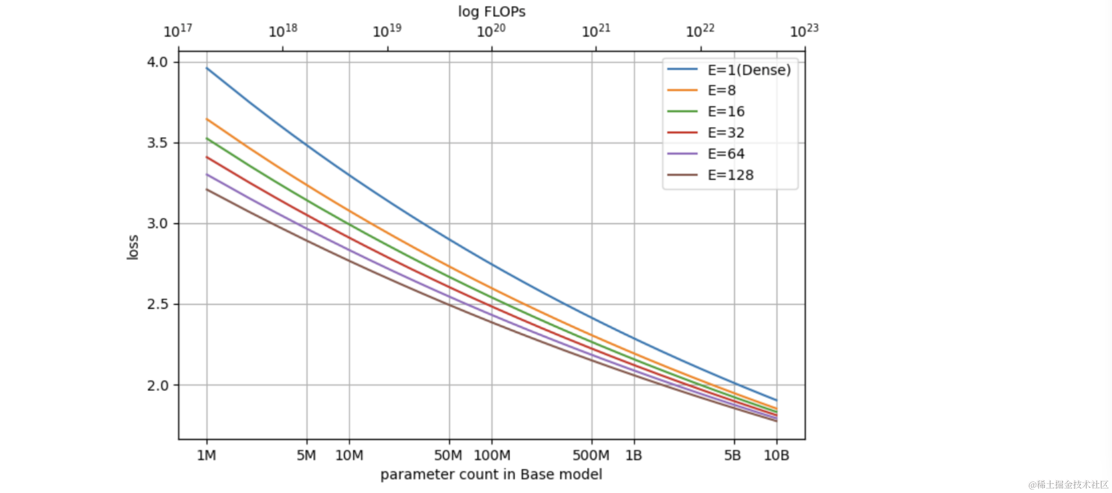
MoE的scaling law建模出自论文 Unified Scaling Laws for Routed Language Models, DeepMind, Feb 2022,关键的工作是基于Dense网络的scaling law,并结合MoE的实验特性,设计出新的建模。
关键假设:MoE模型收敛后(如果没有特殊说明,后续所有的loss都是指收敛后的)的log-loss,是基底参数两log和expert数量log的双线性组合。
表示公式如下:
$$ log L(N, E)\triangleq a\ log\ N + b\ log\ \hat{E} + c\ log\ N log \hat{E} + d \tag{2} $$
$$ where\ \ \ \ \frac{1}{\hat{E}} \triangleq \frac{1}{E-1+(\frac{1}{E_{start}}-\frac{1}{E_{max}})} + \frac{1}{E_{max}} $$
注意:其中 $log$ 函数使用的基底为10。
解释一下其中使用到的变量:
- $E$ 表示expert的数量,$\hat{E}$ 表示饱和化的 $E$,用来衡量expert数量变大后效果变差的衰减;
- $N$ 表示对应基底模型的参数量;
- $a,b,c,d,E_{start},E_{max}$ 为待拟合的参数;
建模方式的演进
下面介绍如何从公式(1)一步步到公式(2)的,以及对应的逻辑。
理论推导部分
如果给定$N$,那么$E$一定程度上与整体参数量成正比;
很容易想到
$$ log\ L_N(E)\triangleq b\ log\ E + d’ \tag{3} $$
$E=1$的时候代表了Dense网络的情况;
带入公式3得到了$log\ L_N(E)= d’$,所以有$d’=a\ log \mathit N + d$;
由此可以得到公式1和公式3的结合:
$$ log\ L(N,E)\triangleq a\ log\ N + b\ log\ E + d \tag{4} $$
到这一步,基于推论的建模就到头了,后续改动都是通过实验观察得到的。
实验修正部分
观察1:公式4在拟合过程中,$b$会随着模型参数增大而增大。
反映了基底模型越大的时候,expert增加带来收益的下降趋势。而在公式4中,$log N$对应的斜率是固定的$a$,因此存在误差。
实验中发现斜率变化与$log\ N$大概成正比,如下图:

所以增加一项$log\ N$与$log\ E$的交叉特征,得到公式5。
$$ log\ L(N,E)\triangleq a\ log\ N + b\ log\ E + c\ log\ N\ log\ E + d \tag{5} $$
此时$log\ E$对应的斜率为$b+c\ log\ N$,如果c为正数那么$N$增大会让斜率增大,既log-loss下降的速度降低。所以一个好的MoE的方法应该让$c$尽量接近于0。
观察2:因为MoE方法中的特性,$E$过大和过小都会影响模型的效果;
比如:
- 如果E多大的时候,会遇到gradient方差变大的情况(expert之间差异比较大),从而降低模型效果;
- 如果E特别小的时候,固定的负担(指负载平衡loss)的影响会更明显,可能影响模型效果;
因此对$E$进行饱和化处理,公式为
$$ \frac{1}{\hat{E}} \triangleq \frac{1}{E-1+(\frac{1}{E_{start}}-\frac{1}{E_{max}})} + \frac{1}{E_{max}} $$
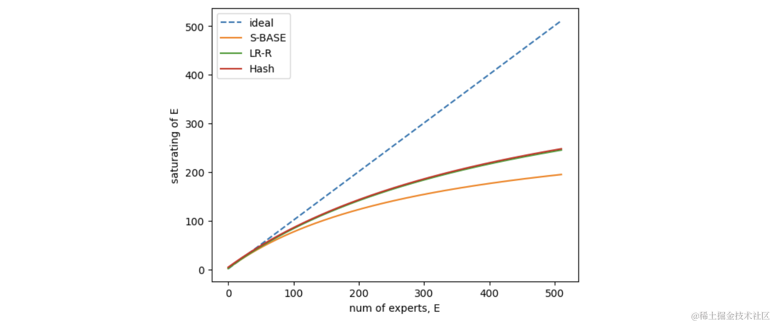
主要特性是$E\to1, \hat{E}\to E_{start}$,$E\to \infty, \hat{E}\to E_{max}$。
取,画出$E$从1到512过程中$\hat{E}$的变化,可以看到当$E$增大的时候,$\hat{E}$增加变缓 代表了增大expert数量带来的收益逐渐降低。因此,在实际使用MoE时,尽量设置不超过128的expert数量。
至此,得到最终的scaling law建模,即公式(1)。另外,因为我们的实验以及场景都是在小于128的场景下进行的,所以饱和化带来的收益比较小,因此,可以沿用论文中的$E_{max}$和$E_{start}$设置,所需需要拟合的参数只有$a,b,c,d$ 这4个。
论文中最终拟合的参数如下:

等价有效参数
通过最终拟合的scaling law,可以计算出MoE设定下对应相同效果的Dense模型参数。
计算过程很简单,解方程:$L(\bar{N}, 1)=L(N, E)$。
得到解:
$$ \bar N \triangleq (N)^{\alpha(\hat{E})/\alpha(E_{start})} (\hat{E}/E_{start})^{b/\alpha{E_{start}}} $$
显而易见,EPC可以带入Dense网络的scaling law计算。
EPC计算代码如下:
import numpy as np
# compute EPC有效参数
E = 16 # Number of Experts
N = 7_241_728_000 # Parameter Count in Base Model

def compute_EPC_by_law(N, E):
    a, b, c, d = -0.082, -0.108, 0.009, 1.104
    e_start, e_max = 1.847, 314.478
    log = np.log10
    def alpha(e):
        return a + c * log(e)
    E_saturating = 1 / (1 / (E-1+1/(1/e_start-1/e_max)) + 1 / e_max)
    factor1 = np.power(N, alpha(E_saturating) / alpha(e_start))
    factor2 = np.power(E_saturating / e_start, b / alpha(e_start) )
    return factor1 * factor2
通过这个公式可以计算得到一系列MoE模型设定下对应的Dense网络表,如下:
| base参数 | expert数量(等价dense参数量) |
|---|---|
| 10M | 8(23.88M), 16(33.89M), 32(48.12M), 64(67.24M), 128(90.77M) |
| 50M | 8(105.73M), 16(142.87M), 32(193.16M), 64(257.59M), 128(333.41M) |
| 100M | 8(200.66M), 16(265.50M), 32(351.46M), 64(459.33M), 128(583.90M) |
| 300M | 8(554.00M), 16(708.92M), 32(907.58M), 64(1.15B), 128(1.42B) |
| 500M | 8(888.35M), 16(1.12B), 32(1.41B), 64(1.76B), 128(2.14B) |
| 800M | 8(1.37B), 16(1.70B), 32(2.12B), 64(2.60B), 128(3.14B) |
| 1B | 8(1.69B), 16(2.08B), 32(2.57B), 64(3.14B), 128(3.76B) |
| 3B | 8(4.65B), 16(5.55B), 32(6.63B), 64(7.85B), 128(9.13B) |
| 5B | 8(7.46B), 16(8.77B), 32(10.30B), 64(12.02B), 128(13.80B) |
| 7B | 8(10.19B), 16(11.85B), 32(13.78B), 64(15.91B), 128(18.11B) |
| 13B | 8(18.05B), 16(20.60B), 32(23.51B), 64(26.68B), 128(29.87B) |
| 70B | 8(85.59B), 16(92.80B), 32(100.62B), 64(108.71B), 128(116.51B) |
| 130B | 8(151.69B), 16(161.39B), 32(171.74B), 64(182.23B), 128(192.18B) |
| 200B | 8(225.88B), 16(237.21B), 32(249.12B), 64(261.05B), 128(272.23B) |
[!important]
应当注意,计算过程中使用的是论文中的数据,可作为参考不代表最终效果!
最终我们期望得到这样的一组scaling law图表,用来指导后续的结构选型。